Analytic variability and multiverse analysis
Better Code, Better Science: Chapter 9, Part 7

This is a possible section from the open-source living textbook Better Code, Better Science, which is being released in sections on Substack. The entire book can be accessed here and the Github repository is here. This material is released under CC-BY-NC-ND.
It’s rarely the case that there is a single analysis workflow that is uniquely appropriate for any particular scientific problem. Different methods come with different assumptions and often embody tradeoffs between different factors:
Bias-variance tradeoffs: While unbiasedness is widely thought to be an important feature of a statistical estimate, we are often willing to trade a small amount of bias in exchange for a significant reduction in the variance of our estimates. The most common example of this is the use of regularized methods that penalize model complexity; for example, regularized regression methods like ridge regression penalize the magnitude of model parameters and thus bias model parameters towards zero in exchange for potentially increased predictive performance.
Penalization tradeoffs: If one uses regularized models then there are tradeoffs in the selection of methods for model fitting (such as L1- versus L2-based penalizations, which vary in the sparseness of their model parameters). Similarly, model comparison methods (such as the use of Akaike Information Criterion (AIC) versus Bayesian Information Criterion (BIC) in model selection) differ in the degree to which they include sample size in the penalty.
Statistical assumptions: Many statistical techniques make assumptions about the distribution of the model residuals or independence of samples.
Sensitivity/specificity tradeoffs: Depending on the application we may worry more about false positives (e.g. disease diagnosis where the treatment is very risky) or false negatives (disease diagnosis where early treatment is the key to survival), and thus we may want to prioritize sensitivity or specificity.
Preprocessing tradeoffs: Preprocessing operations such as smoothing can have important impacts on the data, improving sensitivity to larger features but reducing sensitivity to features smaller than the smoothing operator.
Interpretability tradeoffs: Simple models (such as regularized regression models or decision trees) can be easily interpreted based on the parameter values, but they may not perform as well as more complex models (such as deep neural networks) that can be much more difficult to interpret.
Robustness tradeoffs: In some cases we may want to trade off some degree of sensitivity in favor of robustness. For example, parametric statistical methods are generally more efficient than nonparametric methods when their assumptions are fulfilled, but nonparametric methods provide robustness to failed assumptions at a slight cost of efficiency.
In each of these there is no answer that is universally right: the choices for any application will depend upon the goals of the researcher and the specifics of the data themselves. The goal of sensitivity analysis is to broadly test the range of reasonable/plausible analyses and assess the degree to which the outcomes change in relation to specific analytic choices.
Previous work has shown that real-world analytic variability can have major impact on the results. We (Botvinik-Nezer et al. 2020) examined this in a study that collected a neuroimaging dataset and distributed it to a large number of research teams, asking them to test a set of hypotheses using their standard methods. The results from 70 teams showed a substantial degree of variability; for 5 of the 9 hypotheses tested, the proportion of teams reporting a positive result ranged from 20-40%. The realization of the impact of analytic variability has led to the use of multiverse analysis strategies, in which multiple analytic choices are compared and their impact on the results is assessed.
10.5.1 An example of multiverse analysis
Here I will use an open ecology dataset to ask a simple question: How do bill depth and bill length covary in penguins? This might seem like an obvious question, but it’s actually an example where multiverse analysis can provide useful insight. Gorman and colleagues (Gorman et al. 2014) collected data over three years that included measurements of bill length and depth and body mass from a total of 333 Antarctic penguins, and openly shared those data. The dataset includes three different species of penguins (Adelie, Gentoo, and Chinstrap), each of which inhabits a different ecological niche and has different body characteristics. For this multiverse analysis I focused on two features of the model. First, I varied the way that species is included in the model, either leaving it out of the model, or modeling it using a mixed-effect linear model with either a random intercept or random slope and intercept across species. Second, I varied the inclusion of a number of possible covariates of interest: sex, year of data collection, island where the data were collected, and overall body mass.
One of the challenges of multiverse modeling is organizing all of the different models to be tested, which in this case comprises a set of 48 models. I generated a class that specified all of the model features, and included a method that fits the specified model and returns the results as a dictionary. I then iterated over each modeling approach with all possible combinations of covariates, fitting each of the 48 models, which took about one second to run on my laptop. One common challenge with mixed effects models is that more complex models (like random-slope models) can fail to converge when they are fitted (since they use maximum likelihood estimation and thus must be estimated using optimization), and I saw this initially when I fit the random-slope models using the default optimizer. Because the resulting parameter estimates are not trustable when the model fails to converge, I added code that tried several different optimizers when convergence failed; this resulted in convergence for all of the models.
Once we have fitted all of the models then we need to summarize the results, and a common way to do this is a specification curve plot. Figure 10.16 shows an example of such a plot for the penguin analysis. Strikingly, we see in the top panel that while most of the models show significantly positive coefficients, a subset of models show significantly negative coefficients! The lower panel shows the features of each of the models, which helps understand the cause of the difference in model parameters: The negative parameters occurred only in models where species was not included in the model.
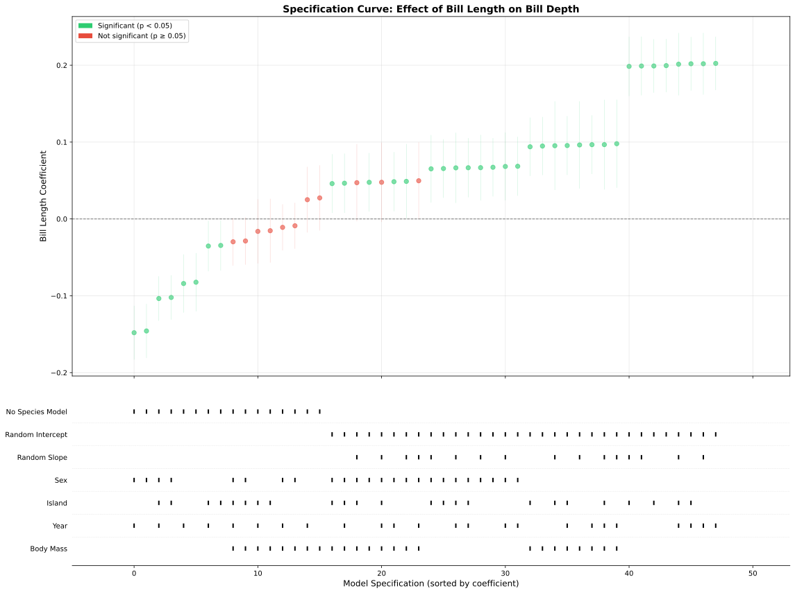
Figure 10.1.6. A specification curve plot for the penguin analysis. The top panel shows the sorted estimated effect sizes for the bill length model parameter across all of the models; statistically significant effects are colored in green. The lower panel shows the features of each model using tick marks.
Figure 10.17 provides further insight into why this occurred. The left panel shows that across all penguins there was a negative relationship between bill length and depth. However, the right panel shows that within each species there was a positive relationship between these features; in the models that included a random effect of species, the overall differences between species were removed and the positive effect could be observed. This is an example of Simpson’s paradox, in which the pattern observed across a dataset is inconsistent with the pattern observed within subgroups of the dataset. This is usually due to the presence of a confounding variable, which in this case is species. This example shows how multiverse analysis can help bring out important features in the data and better understand the robustness of results across modeling choices.
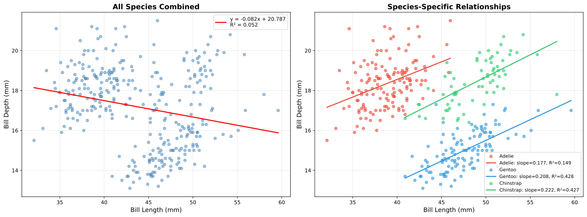
Figure 10.17. Plots showing the regression of bill length against depth in the penguin dataset. The left panel shows the regression computed on the entire dataset combined across all species. The right panel shows separate regressions for each species.
10.5.2 Sensitivity to random seeds
When using analysis methods that involve random numbers, it is essential to establish that the results are robust to different random seeds, and also to determine the degree of variability across simulations due to random seed variability. There is published evidence (Ferrari Dacrema et al. 2021) that some authors may cherry-pick results across random seeds in order to obtain better results, which we sometimes refer to as seed-hacking on analogy to p-hacking. This can be prevented by running an analysis using multiple random seeds and reporting the mean or median along with the variability across seeds.
As an example of how big an impact random seeds can have, I generated 50 synthetic datasets for a classification problem, and assessed the performance of two different classifiers that involve random numbers: a simple neural network model (Perceptron), and a stochastic gradient descent classifier 2. Each classifier was applied to the each dataset using 1000 different random seeds and their accuracy was recorded. The result (shown in Figure 10.18) was striking: although the average performance of the two models differed minimally across the 50,000 simulations (0.7276 for SGD versus 0.7280 for Perceptron), depending on the specific random seed one could find cases where each of the classifiers outperformed the other by almost 10%! This highlights the importance of quantifying the degree of variability due to random seed choice.
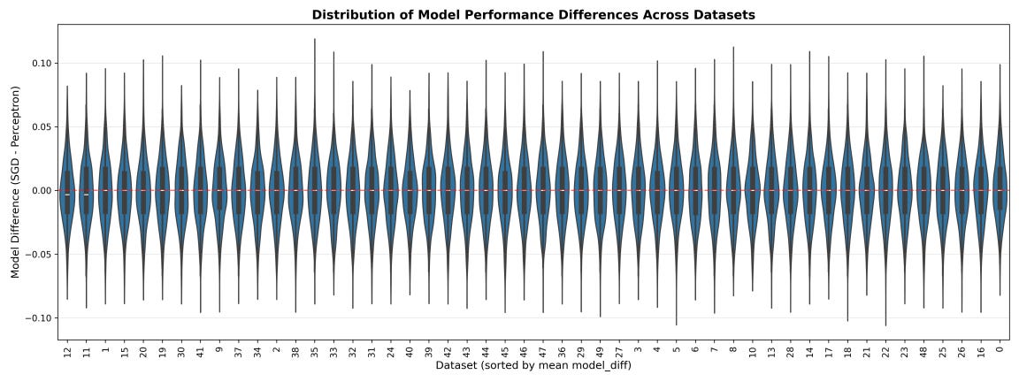
Figure 10.18. A demonstration of variability in classification model accuracy due to different random seeds. Each violin represents the distribution of performance across 1000 random seeds for a single dataset
10.5.3 Sensitivity to modeling assumptions
Statistical models often make assumptions that, if violated, can invalidate any performance guarantees that come with the model. Here we will look at the commonly violated assumption of independence. While assumptions regarding normality of errors are often discussed by researchers, most methods are remarkably robust to violations of normality as long as the sample size is large enough.
Many statistical methods rely upon an assumption that the residuals from the model are independent and identically distributed (or IID). This assumption can easily be violated when the data has structure that involves relationships between observations, such as time-series data, spatial data, clustered data (e.g. data from families), or repeated measures on individuals. When this assumption is violated, the actual error rate of the method can sometimes far exceed the reported error rates computed under the IID assumption (although the parameter estimates should remain unbiased as long as the other assumptions of the model are fulfilled).
10.5.3.1 Clustered data
A common cause of failures of independence is the presence of group structure in the data, which can lead to clustered errors; that is, members of each group are more similar in their errors compared to those in other groups. Figure 10.19 shows how clustering in the data can lead to highly inflated error rates, particularly when there is a small number of clusters. This occurs because clustering leads to underestimation of the standard error that is used to compute the test statistic. There are several different ways that the impact of clustered errors can be corrected, which are differently used across different research domains (McNeish et al. 2017). These include:
Cluster-robust estimators for the standard error (commonly used in biostatistics), which correct the standard error to account for clustering in the data
Fixed effect models (commonly used in economics and social sciences), in which the clustering is modeled out using linear terms
Mixed effect models (commonly used in psychology and social sciences), in which variance components related to clustering are modeled out
Figure 10.19 shows that each of these does a good job of correcting for the effects of clustering in the data. The Python implementation of mixed effects modeling shows slightly inflated error rates, due to the fact that it uses a z-statistic which has slightly inflated error rates for small numbers of clusters, whereas the R implementation uses a correction to the degrees of freedom that corrects this.
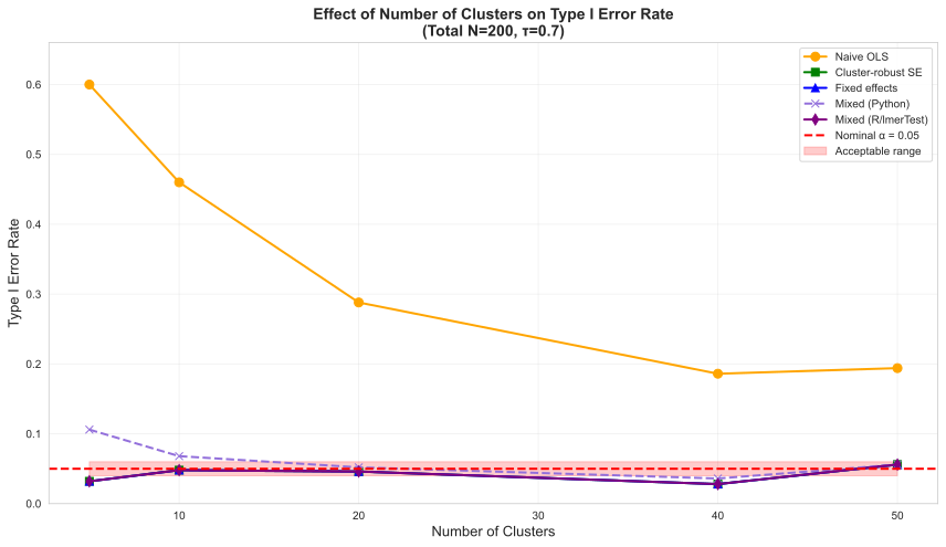
Figure 10.19. An example of the effects of clustering on statistical outcomes. Data were generated with a single intercept for the non-clustered group and with randomly varying intercepts across groups for the clustered group.
10.5.3.2 Autocorrelated data
Even more striking failures to control error can occur when the data are autocorrelated, meaning that adjacent data points in the dataset are correlated, as occurs commonly in timeseries or spatial data. Autocorrelation can severely inflate error rates and render the estimates inefficient, though they generally remain unbiased. Figure 10.20 shows error rates in simulated data with increasing degrees of autocorrelation. The ordinary least squares (OLS) regression model performs very badly here, with false positive rates approaching 70% when autocorrelation reaches 0.9. The results of a number of other methods that are commonly suggested for addressing autocorrelation are also shown in the figure; while these do perform much better than vanilla OLS, none of them appropriately controls error rates as autocorrelation becomes very high. This is a great example of how one can’t simply take the suggestions of a coding agent (or the Internet) and run with them without checking that they adequately control error rates.
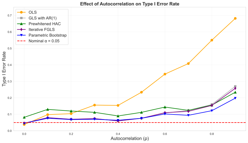
Figure 10.20. An example of the effects of autocorrelation on statistical outcomes. Data were generated with no true signal in the model and with increasing levels of autocorrelation in the noise. In addition to the improper ordinary least squares (OLS) approach, a number of different approaches were applied that are meant to correct for the effects of autocorrelation: generalized least squares (GLS) using an AR(1) covariance, HAC (Heteroskedasticity and Autocorrelation Consistent) standard errors using the Newey-West estimator, iterative feasible generalized least squares (FGLS), and the parametric bootstrap. None of these methods adequately controlled errors when the autocorrelation was high.
This is the final section of the chapter on Validation. In the next set of posts I will turn to performance optimization.