Estimating parameters: Closed-form and Bayesian estimation

Better Code, Better Science: Chapter 9, Part 3

This is a possible section from the open-source living textbook Better Code, Better Science, which is being released in sections on Substack. The entire book can be accessed here and the Github repository is here. This material is released under CC-BY-NC-ND.

It is very common in science to collect data and then use those data to estimate the parameters for a given model, and it’s important to be able to validate that the estimates are valid. Given the central role of parameter estimation in code testing and validation, I now dive into the various methods that one can use to estimate model parameters, and show examples of how we might validate them. In addition to estimating model parameters, we generally also want some kind of way to quantify the uncertainty in our estimates. That is, rather than thinking of the parameter estimate as a single point value, we can ask: What range of values for the parameter are consistent with the data? This is often expressed using confidence intervals, though I will discuss below the ways that these are often misunderstood.

A central idea in this section will be the notion of parameter recovery: that is, how well can our estimation procedure recover the true parameter values using simulated data? This is particularly important in cases where we don’t have statistical guarantees on the unbiasedness of our estimates. As we will see, simulation provides a powerful tool to assess parameter recovery performance for any model.

Closed-form estimates

In some cases parameter estimates can be obtained using a closed form analytic solution. We will use the normal distribution as an example. This distribution has two parameters: a mean (sometimes called a location) that specifies where the center of the distribution falls, and a standard deviation (sometimes called a scale) that specifies the width of the distribution. The probability function for the normal distribution is:

\(p(x \mid \mu, \sigma) = \frac{1}{\sigma \sqrt{2\pi}} \exp\left( -\frac{(x - \mu)^2}{2\sigma^2} \right) \)

where μ is the mean and σ is the standard deviation.

Our goal in estimating model parameters is to find estimates (in this case for the mean and standard deviation) that maximize some measure of goodness of fit with respect to the data, or equivalently, minimize some measure of error. Since we don’t want positive and negative errors to cancel each other out, we need a measure of error that is uniquely positive regardless of the direction of the error. The most common measure in statistics is the mean squared error:

\(\text{MSE} = \frac{1}{n} \sum_{i=1}^{n} (y_i - \hat{y}_i)^2\)

where y_i is the value for the i-th observation, \hat{y_​i​} is the estimated value for that observation from the model, and n is the sample size¹. In the case of the normal distribution, \hat{y_​i​} is the same for each observation: the mean. We can estimate the mean for the sample using the closed form solution:

\(\bar{y} = \frac{1}{n} \sum_{i=1}^{n} y_i \)

​where \bar{y} is the mean. We can then compute the standard deviation using this estimated mean:

\(s_y = \sqrt{\frac{1}{n-1} \sum_{i=1}^{n} (y_i - \bar{y})^2}\)

Note that this is very similar to the mean squared error, differing in the presence of a square root as well as the use of n−1 rather than n in the demominator. The latter is meant to adjust for the fact that we lost one degree of freedom when we estimated the mean from the same data and then used it to compute the standard deviation. When the variance (the square of the standard deviation) is computed using this correction it will be unbiased, meaning that its expected value will match the true variance of the population. The standard deviation is still slightly biased, but less so than the one computed without the correction.

Figure 1 shows an example of a histogram based on samples from a normal distribution, with the theoretical normal distribution based on the estimated sample mean and standard deviation overlaid. Visually it’s clear that the fitted distribution characterizes the overall shape well, even if it mismatches the shape at finer grain, due to sampling variability.

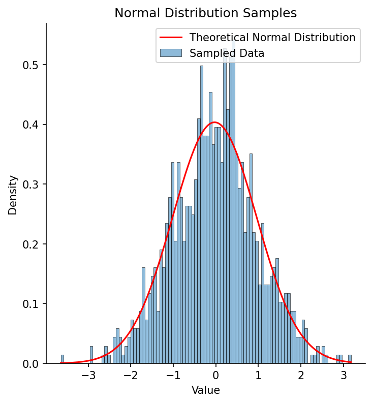
Figure 1. A histogram of 1000 samples from a standard normal distribution (with mean of zero and standard deviation of one), with the fitted normal distribution overlaid in red.

Quantifying uncertainty in closed-form estimation

In general we want not just a point estimate for our parameter but also an estimate of our uncertainty in that estimate. The confidence interval is the most commonly used method for expressing uncertainty around an estimate, and with closed form expressions it’s often possible to compute the confidence interval directly. A confidence interval is expressed in terms of a percentage, but the meaning of this percentage is often misinterpreted (see the discussion in my Statistical Thinking for more on this). The term “95% confidence interval” seems to imply that it is an interval in which we have 95% confidence that the true value of the parameter falls. However, that violates the frequentist statistical logic that underlies the computation of the confidence interval, which treats the true value as fixed, and thus it either falls in the interval or it doesn’t. Instead, the more appropriate interpretation of a frequentist confidence interval is that it is the interval that would capture the true population mean 95% of the time for samples from the same population. I prefer to frame it in a slightly different, if somewhat less precise way: The confidence interval expresses the range of plausible values for the parameter given our data, and thus tells us something about the precision of our estimate: All else being equal, a sample estimate with a narrower confidence interval is more precise than an estimate with a wider confidence interval.

Using our example from above, we can compute a confidence interval for our estimate of the sample mean. This requires that we have a probability distribution that is associated with our statistic; in this case, the Student’s t distribution is appropriate since we have estimated the standard deviation as well as the mean. The t distribution has slightly wider tails than the normal distribution, which helps account for the added uncertainty in our estimate of the standard deviation. The equation for the confidence interval around the mean using the t distribution is:

\(\bar{y} \pm t_{\alpha/2, \, n-1} \cdot \frac{s_y}{\sqrt{n}} \)

where s_y​ is the sample standard deviation, n is the sample size, and t_α/2,n−1​ is the critical value of the t distribution with n−1 degrees of freedom at the α/2 percentile. α defines our confidence level, and it is divided by two since we are interested in both the positive and negative directions. In our case, this results in a confidence interval of [-0.09028, 0.03249]. We can use a simulation to confirm that this interval indeed captures the sample mean 95% of the time for new samples from the same distribution:

# Simulation parameters
n_simulations = 100000
confidence_level = 0.95
alpha = 1 - confidence_level
random_state = 42
true_mean, true_sd = 0, 1
sample_size = 1000

# Track how many times the CI captures the true mean
captures = 0

# Run simulations
for i in range(n_simulations):
    # Draw a new sample from the population
    sample = norm.rvs(loc=true_mean, scale=true_sd, 
        size=sample_size, random_state=random_state)
    
    # Calculate sample statistics
    sample_mean_sim = np.mean(sample)
    sample_sd_sim = np.std(sample, ddof=1)
    
    # Calculate confidence interval
    df = sample_size - 1
    t_crit = t.ppf(1 - alpha/2, df)
    se = sample_sd_sim / np.sqrt(sample_size)
    margin = t_crit * se
    
    ci_low = sample_mean_sim - margin
    ci_high = sample_mean_sim + margin
    
    # Check if CI captures the true mean
    if ci_low <= true_mean <= ci_high:
        captures += 1

# Calculate coverage rate
coverage_rate = captures / n_simulations

print(f"Simulation results:")
print(f"Number of simulations: {n_simulations}")
print(f"Sample size per simulation: {sample_size}")
print(f"True population mean: {true_mean}")
print(f"Confidence level: {confidence_level * 100}%")
print(f"\nCoverage rate: {coverage_rate:.4f} ({coverage_rate * 100:.2f}%)")

Simulation results:
Number of simulations: 100000
Sample size per simulation: 1000
True population mean: 0
Confidence level: 95.0%

Coverage rate: 0.9503 (95.03%)

Here we see that the observed proportion of samples where the sample mean falls within the confidence interval is very close to the 95% that we expect based on statistical theory.

The bootstrap as a general method for quantifying uncertainty

There are often cases where we don’t have a sampling distribution that we can use to form a confidence interval. In these cases, we can use a technique known as the bootstrap. This method takes advantage of resampling, meaning that we repeatedly draw samples with replacement from our full sample. We can do this using the scipy.stats.bootstrap() function, which performs the bootstrap on a sample given any statistical function:

from scipy.stats import bootstrap

# use the bias-corrected/accelerated method ('BCa')
res = bootstrap((normal_samples,), np.mean, confidence_level=0.95,      
    n_resamples=10000, method='BCa', random_state=random_state)

print(f'Bootstrap 95% CI for mean: '
    f'[{res.confidence_interval.low:.5f}, '
    f'{res.confidence_interval.high:.5f}]')
print(f'CI based on t-distribution: [{ci_lower:.5f}, {ci_upper:.5f}]')

Bootstrap 95% CI for mean:  [-0.09104, 0.03078]
CI based on t-distribution: [-0.09028, 0.03249]

Here we see that the bootstrap procedure gives results that are very close to those obtained using the closed form solution, but has the advantage of being usable with nearly any statistic (except for those based on extreme values) regardless of whether or not there is a closed form estimator and/or the sampling distribution is analytically tractable.

Bayesian estimation

I noted above that the interpretation of the frequentist confidence interval is counterintuitive for most people, which leads to common misunderstandings, even among experts (Hoekstra et al., 2014). We would like a way of generating an interval that expresses our confidence about the true parameter value, but we can’t do this in the frequentist framework. However, there is a different approach to statistics that allows us to generate such an interval, known as Bayesian statistics after the Reverend Thomas Bayes whose famous equation forms the basis of this approach.

Bayesian statistics is based on a different conception of probability from the frequentist approach that underlies the standard confidence interval. Under the frequentist conception, probabilities are meant to refer to the long-run frequencies of outcomes across many samples, while the true parameter value is viewed as fixed. For this reason, it doesn’t make sense to a frequentist to say that there is a particular probability of the true parameter value; it simply is what it is. Bayesians, on the other hand, view probabilities as degrees of belief, and treat the estimation of parameters from data as a way to sharpen our belief - that is, as a learning opportunity. This means that it is perfectly legitimate in the Bayesian framework to say that there is a 95% probability that the true value of a parameter lies within a particular interval.

The fundamental idea in Bayesian statistics is that we start with a set of beliefs (known as a prior distribution), we obtain some relevant data, and then use the likelihood of those data given the possible parameter values to update our beliefs, generating a posterior distribution. I won’t go into detail about Bayesian methods here; see my Statistical Thinking for a basic overview, and Gelman et al. (2013) or McElreath (2020) for more detailed overviews. Instead I will show an example of Bayesian estimation applied to our example data above. There are several Python packages that can be used to perform Bayesian estimation; I will use the popular PyMC package. The first section sets up the Bayesian model, with priors for the mean (mu) and standard deviation (sigma) that are very broad and thus will have little influence on the outcome; in Bayesian terms these are referred to as weakly informative priors. We then perform sampling to obtain an estimate of the posterior distribution of the parameters given the data. Using these distributions, we can then find the narrowest set of values that contain 95% of the mass of posterior distribution, which are known as the highest density interval (HDI) (which is a type of credible interval that contains the most likely values). This interval serves as a Bayesian alternative to the frequentist confidence interval, allowing us to legitimately describe it as the interval that has a 95% probability of containing the true value.

import pymc as pm
import arviz as az

# Bayesian estimation using PyMC
with pm.Model() as model:
    # Priors for unknown model parameters
    mu = pm.Normal('mu', mu=0, sigma=1000)  # Prior for mean
    sigma = pm.HalfNormal('sigma', sigma=100)  # Prior for standard deviation (must be positive)
    
    # Likelihood (sampling distribution) of observations
    likelihood = pm.Normal('likelihood', mu=mu, sigma=sigma, observed=normal_samples)
    
    # Posterior sampling
    trace = pm.sample(10000, tune=1000, return_inferencedata=True, random_seed=42)

# Extract posterior estimates
posterior_mean = trace.posterior['mu'].mean().values
posterior_sd = trace.posterior['sigma'].mean().values

# extract highest density interval
hdi = az.hdi(trace, hdi_prob=0.95)
hdi_values = hdi.mu.values

print(f"Posterior mean: {posterior_mean:.5f}, Posterior sd: {posterior_sd:.5f}")
print(f"Sample mean: {sample_mean:.5f}, Sample sd: {sample_sd:.5f}")
print(f'95% HDI values: {hdi_values}')
print(f'95% CI based on t-distribution: [{ci_lower:.5f}, {ci_upper:.5f}]')

Posterior mean: -0.02895, Posterior sd: 0.99033
Sample mean: -0.02889, Sample sd: 0.98922
95% HDI values:                 [-0.08993, 0.03335]
95% CI based on t-distribution: [-0.09028, 0.03249]

In this case, the Bayesian HDI turns out to be very close to the parametric confidence interval. We can also obtain a visualization of the full posterior distributions obtained through Bayesian estimation, which are shown in :

# Visualize posterior distributions
fig, axes = plt.subplots(1, 2, figsize=(12, 4))

# Plot posterior for mu
az.plot_posterior(trace, var_names=['mu'], ax=axes[0])
axes[0].axvline(sample_mean, color='red', linestyle='--', label='Sample mean')
axes[0].legend()

# Plot posterior for sigma
az.plot_posterior(trace, var_names=['sigma'], ax=axes[1])
axes[1].axvline(sample_sd, color='red', linestyle='--', label='Population sd')
axes[1].legend()

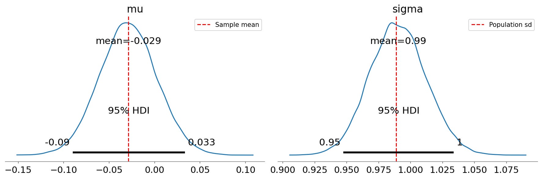
Figure 2. Posterior distributions for mean (mu) and standard deviation (sigma) obtained using Bayesian estimation, with the 95% highest density interval shown by the gray bar at the base of the plot.

Bayesian estimation can be particularly useful when one has a strong prior belief about the value of a parameter and wishes to update that belief based on data. For example, let’s say that there was a published dataset that reported a particular parameter value, and a researcher performs additional observations and wants to update that parameter estimate. Bayesian estimation allows this by the specification of the prior probability distribution. In the example above we used a relatively non-informative prior for the mean (a normal distribution with mean of zero and standard deviation of 1000, which allows for a very wide set of possibilities). However, if we have existing data then we can use those data to inform our subsequent analyses, consistent with the idea that Bayesian inference is a form of learning from data. One can also provide a prior based on one’s scientific hypotheses or expectations, and the ability to incorporate prior knowledge into parameter estimation is generally taken as a strength of Bayesian methods; however, one must be sure that the prior doesn’t overwhelm the data dogmatically, effectively forcing a particular answer regardless of what the data say.

One drawback of Bayesian methods is that they can be very computationally expensive. For example, the Bayesian estimation above took a bit over 2 seconds using 4 parallel sampling processes, which is much slower than the 189 microseconds required for closed-form estimation and also substantially slower than the optimization methods discussed in the next section. There are alternative Bayesian methods known as variational Bayes that use mathematical tricks to speed up estimation, but often require substantial mathematical skill to develop, though some packages like PyMC now offer built-in variational Bayes methods.

In the next post I will turn to parameter estimation using optimization methods.

1. I apologize for the wonky formatting of the mathematical features in the text, unfortunately Substack doesn’t seem to support in-line LaTeX formatting.