Estimating parameters using optimization
Better Code, Better Science: Chapter 9, Part 4

This is a possible section from the open-source living textbook Better Code, Better Science, which is being released in sections on Substack. The entire book can be accessed here and the Github repository is here. This material is released under CC-BY-NC-ND.
In many cases we don’t have a closed form solution that we can use to compute the parameter estimates directly. In this case it’s common to use some form of optimization (or search) process to find the parameters that best fit the data. The simplest way to do this is to try a large range of parameter values and choose the one that best fits the sample, which is known as a grid search. This is generally done with the goal of maximizing the likelihood of the data given the model parameters, and hence is called maximum likelihood estimation. In other words, we aim to find the values of the parameters that make the observed data most likely. In practice we would generally use the log of the likelihood rather than the likelihood itself, since these values are often very small which can result in floating point errors.
In the case of the normal distribution the maximum likelihood estimate is equivalent to the estimate that minimizes the squared error, since the sample variance (which is based on the squared error) is part of the likelihood equation. But we can also use this example to see how grid search might work with our sample. I ran a grid search using a grid of 1000 possible mean values linearly spaced across [-1, 1], and 1000 possible standard deviation values spaced across [0.5, 1.5]; these particular values were based on my knowledge that the data came from a normal distribution and that these ranges should be likely to capture the parameter values in a dataset of this size. The results came out very close to those obtained using the closed-form solution; note that the maximum likelihood estimate for the standard deviation is equivalent to the population rather than sample standard deviation (i.e. it uses NN rather than N−1N−1 in its denominator), so I corrected the sample standard deviation to make the comparison fair:
Best fit mean: 0.0190,   Best fit sd: 0.9785, loglik: -1397.4353
Sample mean:   0.0193, Population sd: 0.9787, loglik: -1397.4352
We can see this visualized in Figure 1, where we see the landscape of the likelihood across a range of possible parameter values; here we use the negative log-likelihood for visualization, since optimization methods tend to use the language of minimization rather than maximization. We can see that this landscape is smooth and only has one visible minimum; this occurs because the negative log-likelihood surface for the normal distribution is convex, which guarantees that there is a single minimum and thus that regardless of where we start our search, we are guaranteed to find the global minimum by simply following the surface downward, a process central to many optimization algorithms (including the commonly used gradient descent). As we will see below, most realistic optimization problems have multiple local minima, making them much more difficult to optimize by simply following the surface downward.
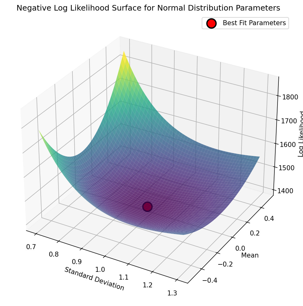
Figure 1. A visualization of the negative log-likelihood landscape for a range of parameter values in the grid search for the mean and standard deviation of a normal distribution.
While grid search worked, it was exceedingly slow, taking more than 25 seconds to estimate the parameters that were estimated by closed form in less than a millisecond - a staggering 89,000 times slower! Grid search is inefficient even with just two parameters, and becomes exponentially less efficient with each additional parameter. A more effective and efficient way to estimate parameters is using optimization methods that are specifically built to search for parameter values that minimize a particular loss function. A common choice in Python is scipy.optimize.minimize(), which offers a number of algorithms for parameter search. We can implement this for our normal distribution data; because the function finds the minimum, we will use the negative log-likelihood as our target, which is equivalent to maximizing the log-likelihood:
import time
from scipy.stats import norm

def negative_log_likelihood(params, data):
    """Negative log likelihood function to minimize"""
    mu, sd = params
    # ensure sd is positive to avoid dividing by zero
    if sd <= 0:
        return np.inf
    return -norm.logpdf(data, loc=mu, scale=sd).sum()

# initial guess
initial_params = [0, 1]

start_time = time.time()
result = minimize(negative_log_likelihood, initial_params, args=(normal_samples,),
                  method='Nelder-Mead')
This gives us a solution that is equal to the fourth decimal place:
Optimized mean: 0.01926,  Optimized sd: 0.97873, loglik: -1397.43520
Sample mean:    0.01933, Population sd: 0.97873, loglik: -1397.43519
These estimates were obtained about 8,000 times more quickly compared to grid search, though still about 10 times slower than the closed-form solution. Note that I had to add some initial guesses for our parameter values, and for this example I used values that were close to the known true values. However, even when the starting values are far from the true values, optimization can often find them quickly and effectively. For example, setting the starting points for both mean and standard deviation to 10,000, the resulting parameter estimates were basically identical, and it still completed more than 2,700 times faster than the grid search.
It’s common to put boundaries on an optimization when there are bounds outside which we are sure that the parameter shouldn’t go. For example, in our example we know that the standard deviation cannot be negative, so we could set the lower bound on the standard deviation parameter to just above zero:
from scipy.optimize import minimize, Bounds

bounds = Bounds(lb=[-np.inf, 1e-6], ub=[np.inf, np.inf])
result = minimize(negative_log_likelihood, initial_params, args=(normal_samples,),
                  method='L-BFGS-B', bounds=bounds)
This doesn’t have much impact on this particular problem, but with complex models and multiple parameters it’s common for parameter values to explode, and setting boundaries can help prevent that. However, as I will discuss below, it’s important to ensure that parameter estimates don’t sit at the boundaries, as this can suggest pathologies in model fitting.
Automated differentiation
The optimization methods discussed above are limited either to small numbers of parameters (like derivative-free methods such as Nelder-Mead) or small numbers of data points (like gradient-based methods such as L-BFGS that require computation of gradients across the entire dataset on each optimization step). Given this, how is it possible to train artificial neural networks that may have billions of parameters over trillions of data points? A key innovation that has enabled effective training of large models is automatic differentiation (often called autodiff for short) combined with gradient descent. Automatic differentiation takes a function definition and (when possible) automatically determines the derivatives of the loss function with respect to the parameters. Gradient descent uses those derivatives to follow the loss landscape downwards. In deep learning it’s most common to use stochastic gradient descent (SGD), which uses small mini-batches of data to iteratively estimate the gradients; even though the estimates for each individual batch are noisy, they are unbiased estimates of the true gradient and computationally cheap to obtain, such that the noise averages out over many iterations to give precise parameter estimates at comparatively low computational cost. However, given the small dataset in this sample we will use the simpler standard gradient descent over the entire dataset at once.
As an example, we can estimate parameters for the Michaelis-Menten equation from biochemistry, which describes the rate at which an enzyme converts its substrate into its product:
where V is the reaction velocity, S is the concentration of the enzyme’s substrate, V_max is the maximum reaction velocity once the enzyme is saturated with substrate, and K_m is the Michaelis constant that describes the affinity of the particular enzyme for its substrate (defined as the value of SS at which V=Vmax/2V=Vmax/2). Figure 2 shows a plot of this function for the acetylcholinesterase enzyme, along with noisy data generated from the function.
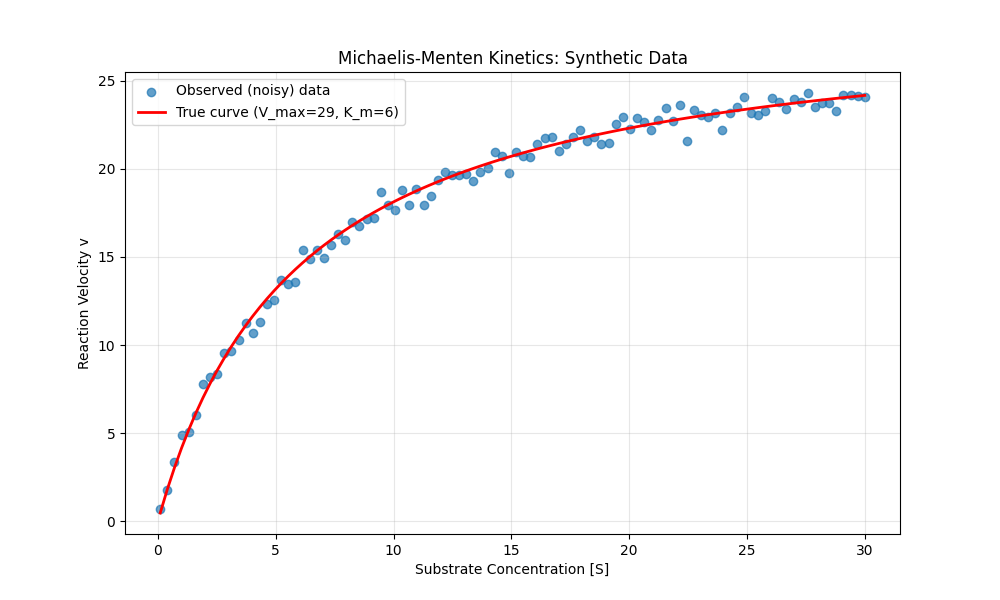
Figure 2. A plot of the Michaelis-Menten function for acetylcholinesterase, along with data sampled from this function with added Gaussian random noise.
This equation could easily be solved using simpler methods, but it’s a nice simple example to show how model parameters can be estimated using autodiff with gradient descent. We can start by defining the Michaelis-Menten function and generating some data with random noise (shown in ; plotting code omitted):
def michaelis_menten(S, V_max, K_m):
    return (V_max * S) / (K_m + S)

V_max_true = 29  # Maximum velocity (in nM/min)
K_m_true = 6     # Michaelis constant (in mM)
noise_sd = 0.5    # Standard deviation of noise

# Generate substrate concentration data points
S = np.linspace(0.1, 30, 100)

v_true = michaelis_menten(S, V_max_true, K_m_true)
noise = np.random.normal(0, noise_sd, size=v_true.shape)
v_observed = v_true + noise
In order to invoke the automatic differentiation mechanism in PyTorch, we simply need to specify requires_grad=True for the variables that we intend to estimate:
# Convert data to PyTorch tensors
S_tensor = torch.tensor(S, dtype=torch.float32)
v_observed_tensor = torch.tensor(v_observed, dtype=torch.float32)

# specify initial guesses
V_max_init = 10.0
K_m_init = 10.0

# Initialize parameters with random guesses
# requires_grad=True enables automatic differentiation
V_max = torch.tensor(V_max_init, requires_grad=True)
K_m = torch.tensor(K_m_init, requires_grad=True)
We also need to set up a loss function that will define how far the prediction is from the data, for which we will use the squared error:
def compute_loss(V_max, K_m, S, v_observed):
    """Compute MSE loss between predicted and observed velocities."""
    v_predicted = michaelis_menten(S, V_max, K_m)
    loss = torch.mean((v_predicted - v_observed) ** 2)
    return loss
Using this we set up our training loop that uses gradient descent to estimate the parameters (with some code omitted for clarity), and assess the parameter recovery of the model by comparing the estimates to the true values:
# Hyperparameters
learning_rate = 0.1
n_iterations = 500

# Test the loss with initial parameters
initial_loss = compute_loss(V_max, K_m, S_tensor, v_observed_tensor)
print(f"Initial loss: {initial_loss.item():.4f}")

# Gradient descent training Loop
for i in range(n_iterations):
    # Forward pass: compute loss
    loss = compute_loss(V_max, K_m, S_tensor, v_observed_tensor)

    # Backward pass: compute gradients via autodiff
    loss.backward()

    # Update parameters using gradient descent step
    # torch.no_grad() prevents these operations from being tracked
    with torch.no_grad():
        V_max -= learning_rate * V_max.grad
        K_m -= learning_rate * K_m.grad

        # Zero the gradients for the next iteration
        V_max.grad.zero_()
        K_m.grad.zero_()

print(f"\nFinal estimates: V_max = {V_max.item():.4f}, K_m = {K_m.item():.4f}")
print(f"True values:     V_max = {V_max_true:.4f}, K_m = {K_m_true:.4f}")
Initial loss: 188.0915
Final loss:     0.2006

Final estimates: V_max = 29.0894, K_m = 6.1336
True values:     V_max = 29.0000, K_m = 6.0000
Since there are only two parameters, we can easily visualize how the parameter estimate traverses the loss landscape as the estimation process moves from the initial guesses (in this case 10 for both parameters) to the final values, as shown in Figure 3.
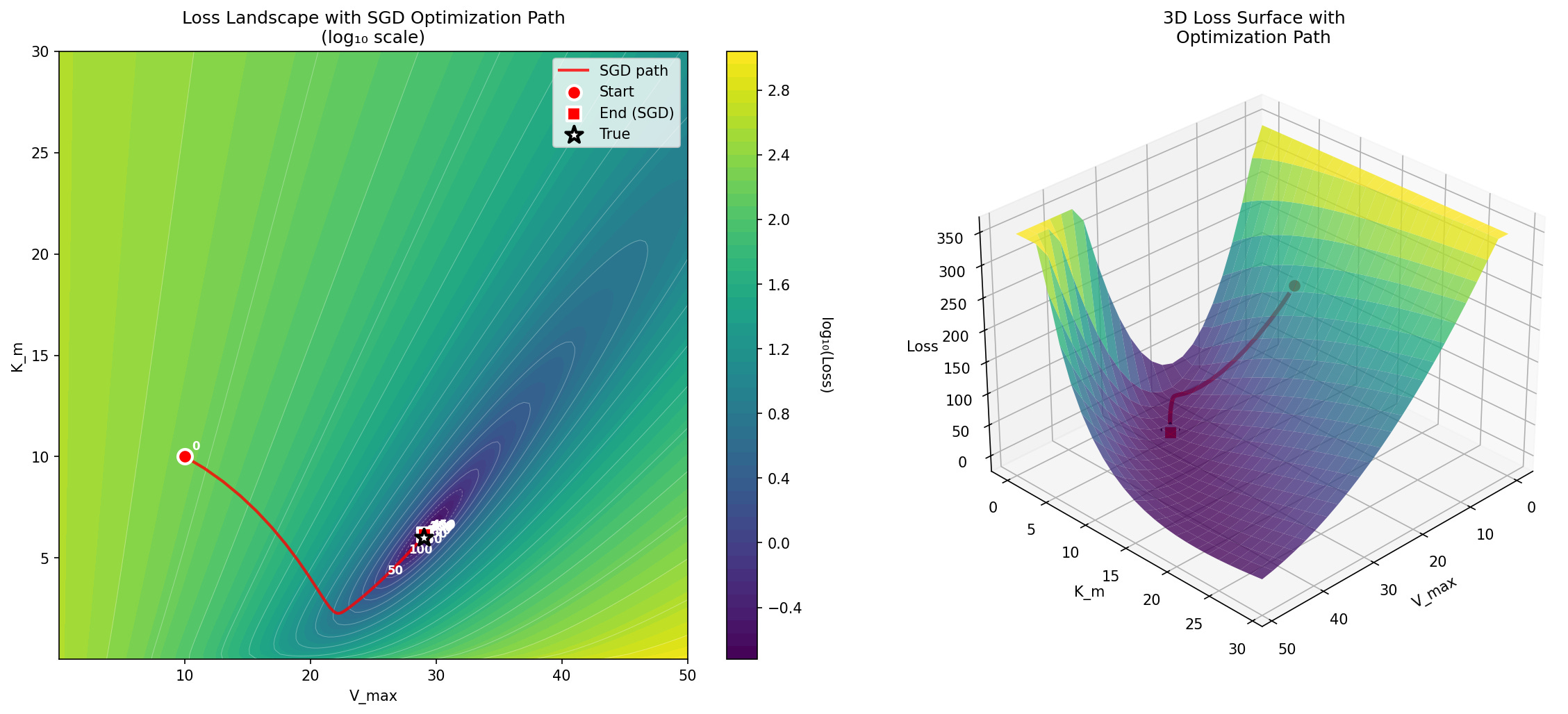
Figure 3. A visualization of the log-loss landscape for the Michaelis-Menten optimization problem, showing the journey of the optimization process from the starting point to the ending point.
Local minima in optimization
The error landscape for the normal distribution example is convex, which means that there is a single global minimum that can be found simply by following the error gradient downwards. Claude Sonnet 4 initially tried to convince me that the Michaelis-Menten problem is convex, but was overruled by Claude Opus 4.5. Despite being non-convex, the error landscape of the Michaelis-Menten problem is smooth and relatively well behaved, as seen in Figure 4. However, many realistic scientific problems have highly complex non-convex likelihoods, such that there are numerous local minima that the optimization routine can get stuck in. shows an example of this.
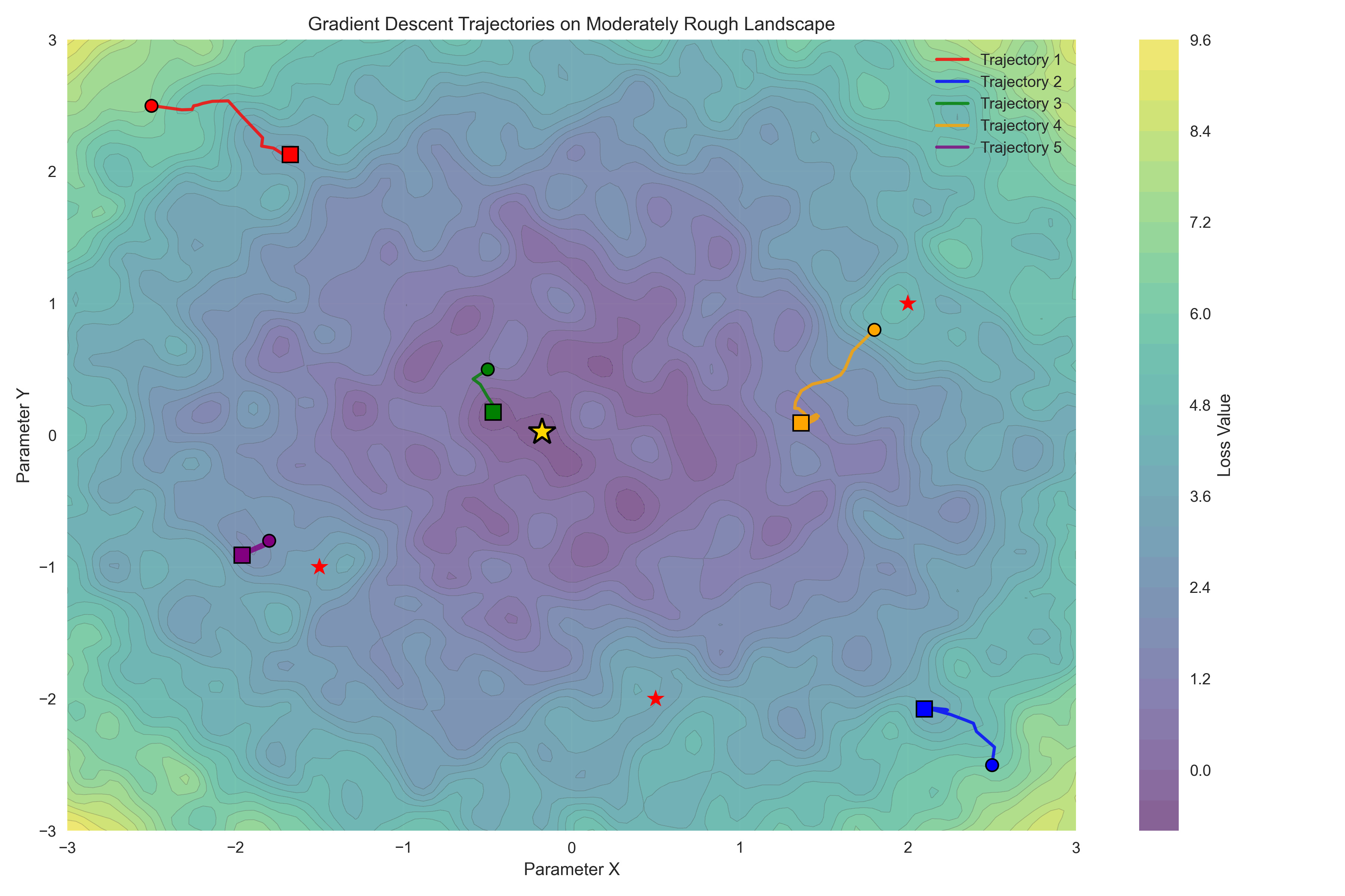
Figure 4. A visualization of a rough loss landscape. The star shows the global minimum, and the individual trajectories show the local minima that are found when using simple gradient descent from different starting points.
There are a number of strategies that one can employ to help avoid parameter estimates that are far from the optimal answer that is located at global loss minimum:
Run the estimation algorithm multiple times with different random initializations of the parameters. If they are similar between runs then this gives confidence that the estimates don’t reflect local minima. If the parameter estimates differ yet losses are similar, this suggests that the parameters may be trading off against one another, which reflects a structural problem with the model or data such that there are many equally good points in the loss landscape. This is often referred to as non-identifiability of the parameters, and is sometimes evident in correlations between the different parameter estimates.
Use an optimizer that adapts the learning rate to the local gradient, such as ADAM or RMSprop.
Use an optimizer that explores more broadly before converging, such as the differential evolution method implemented in
scipy.optimize.differential_evolution.It can sometimes be helpful to reparameterize the model to help with convergence. For example, if the models are physically constrained to being positive, then one might consider optimizing the logarithm of the parameter rather than the natural values of the parameters; this allows the optimizer to explore the entire range of large and small numbers while respecting the positivity constraint. If the different parameters are on very different scales this can also cause problems since the optimizer needs to move at different rates in different directions of the loss space, so reparameterizing the model such that parameters are in roughly the same numeric scale can be useful.
In the next post I will discuss another strategy for parameter estimation known as simulation-based inference.
People in my lab really like optuna. It’s a Python package that automates a lot of these steps - starting from different initial conditions with different seeds.