Managing complex scientific workflows

Better Code, Better Science: Chapter 8, Part 9

This is a possible section from the open-source living textbook Better Code, Better Science, which is being released in sections on Substack. The entire book can be accessed here and the Github repository is here. This material is released under CC-BY-NC-ND.

We now turn to a more realistic and complex scientific data analysis workflow. For this example I will use an analysis of single-cell RNA-sequencing data to determine how gene expression in immune system cells changes with age. This analysis will utilize a large openly available dataset that includes data from 982 people comprising about 1.3 million peripheral blood mononuclear cells (i.e. white blood cells) for about 35K transcripts. I chose this particular example for several reasons:

• It is a realistic example of a workflow that a researcher might actually perform.

• It has a large enough sample size to provide a robust answer to our scientific question.

• The data are large enough to call for a real workflow management scheme, but small enough to be processed on a single laptop (assuming it has decent memory).

• The workflow has many different steps, some of which can take a significant amount of time (over one hour)

• There is an established Python library (scanpy) that implements the necessary workflow components.

• It’s an example outside of my own research domain, to help demonstrate the applicability of the book’s ideas across a broader set of data types.

I will use this example to show how to move from a monolithic analysis script to a well-structured and usable workflow that meets most of the desired features described above.

Note: I am not an expert in RNA-seq analysis. I would welcome comments from experts on the workflow that I have implemented here.

Starting point: One huge notebook

I developed the initial version of this workflow as many researchers would: by creating a Jupyter notebook that implements the entire workflow, which can be found here. The total execution time for this notebook is about two hours on an M3 Max Macbook Pro.

The problem of in-place operations

What I found as I developed the workflow was that I increasingly ran into problems that arose because the state of particular objects had changed. This occurred for two reasons at different points. In some cases it occurred because I saved a new version of the object to the same name, resulting in an object with different structure than before. Second, and more insidiously, it occurred when an object passed into a function was modified by the function internally. This is known as an in-place operation, in which a function modifies an object directly rather than returning a new object that can be assigned to a variable.

In-place operations can make code particularly difficult to debug in the context of a Jupyter notebook, because it’s a case where out-of-order execution can result in very confusing results or errors, since the changes that were made in-place may not be obvious. For this reason, I generally avoid any kind of in-place operations if possible. Rather, any function should immediately create a copy of the object that was passed in, and then do its work on that copy, returning at the end of the function for assignment to a new variable. One can then re-assign it to the same variable name if desired, which is more transparent than an in-place operation but still makes the workflow dependent on the exact state of execution and can lead to confusion when debugging. Some packages allow a feature called “copy-on-write” which defers actually copying the data in memory until it is actually modified, which can make copying more efficient; this feature is becoming the default in pandas.

If one must modify objects in-place, then it is good practice to announce this loudly. The loudest way to do this would be to put “inplace” in the function name. Another cleaner but less loud way is through conventions regarding function naming; for example, in PyTorch it is a convention that any function that ends with an underscore (e.g. tensor.mul_(x)) performs an in-place operation whereas the same function without the underscore (tensor.mul(x)) returns a new object. Another way that some packages enable explicit in-place operations is through a function argument (e.g. inplace=True in pandas), though this is being phased out from many functions in pandas because “It is generally seen (at least by several pandas maintainers and educators) as bad practice and often unnecessary” (PDEP-8).

One way to prevent in-place operations altogether is to use data types that are immutable, meaning that they can’t be changed once created. This is one of the central principles in functional programming languages (such as Haskell), where all data types are immutable, such that one is required to create a new object any time data are modified. Some native data types in Python are immutable (such as tuples and frozensets), and some data science packages also provide immutable data types; in particular, the Polars package (which is meant to be a high-performance alternative to pandas) implements its version of a data frame as an immutable object, and the JAX package (for high-performance numerical computation and machine learning) implements immutable numerical arrays.

Converting from Jupyter notebook to a runnable python script

As we discussed in an earlier chapter, converting a Jupyter notebook to a pure Python script is easy using jupytext. This results in a script that can be run from the command line. However, there can be some commands that will block execution of the script; in particular, plotting commands can open windows that will block execution until they are closed. To prevent this, and to ensure that the results of the plots are saved for later examination, I replaced all of the plt.show() commands that display a figure to the screen with plt.savefig() commands that save the figures to a file in the results directory. (This was an easy job for the Copilot agent to complete.)

Decomposing a complex workflow

The first thing we need to do with a large monolithic workflow is to determine how to decompose it into coherent modules. There are various reasons that one might choose a particular breakpoint between modules. First and foremost, there are usually different stages that do conceptually different things. In our example, we can break the workflow into several high-level processes:

• Data (down)loading

• Data filtering (removing subjects or cell types with insufficient observations)

• Quality control

  • identifying bad cells on the basis of mitochondrial, ribosomal, or hemoglobin genes or hemoglobin contamination

  • identifying “doublets” (two cells captured in a single barcode)

• Preprocessing

  • Count normalization

  • Log transformation

  • Identification of high-variance features

  • Filtering of nuisance genes

• Dimensionality reduction

• UMAP generation

• Clustering

• Pseudobulking (aggregating cells within an individual)

• Differential expression analysis

• Pathway enrichment analysis (GSEA)

• Overrepresentation analysis (Enrichr)

• Predictive modeling

In addition to a conceptual breakdown, there are also other reasons that one might want to further decompose the workflow:

• There may be points where one might need to restart the computation (e.g. due to computational cost).

• There may be sections where one might wish to swap in a new method or different parameterization.

• There may be points where the output could be reusable elsewhere.

Resumable workflows

I asked Claude Code to help modularize the monolithic workflow, using a prompt that provided the conceptual breakdown described above. The resulting code ran correctly, but crashed about two hours into the process due to a resource issue that appeared to be due to asking for too many CPU cores in the differential expression analysis. This left me in the situation of having to rerun the entire two hours of preliminary workflow simply to get to a point where I could test my fix for the differential expression component, which is not a particularly efficient way of coding. The problem here is that the workflow execution was stateful, in the sense that the previous steps need to be rerun prior to performing the current step in order to establish the required objects in memory. The solution to this problem is to implement the workflow in a resumable way, which doesn’t require that earlier steps be rerun if they have already been completed. One way to do this is by implementing a process called checkpointing, in which the intermediate state is stored for each step. These checkpoint files can then be used to start the workflow at any point without having to rerun all of the previous steps.

Another important feature of a workflow related to resumability is idempotency, which means that a workflow will result in the same answer when run multiple times. This is related to, but not the same as, the idea of resumability. For example, a resumable workflow that saves its outputs to cache files could fail to be idempotent if the results were appended to the output file with each execution, rather than overwriting them. This would result in different outputs depending on how many times the workflow has been executed. Thus, when we use caching we should be sure to either reuse the existing file or rewrite it completely with a new version.

When it comes to building a resumable workflow, there are two options:

• Build it from scratch

• Use an existing workflow engine

While there may sometimes be good reasons to build a workflow from scratch (and I actually do so in developing this chapter: see here), one’s first inclination should always be to see whether there is an existing tool that can solve the problem.

Managing a complex workflow with Snakemake

In this example I will focus on the Snakemake workflow engine. Figure 1 shows the DAG generated by Snakemake for the RNA-seq analysis workflow.

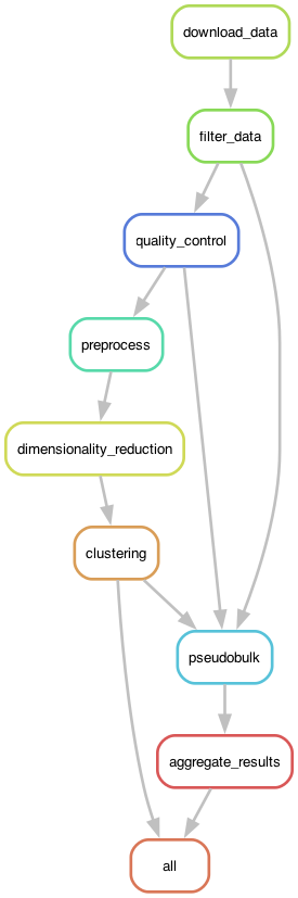
Figure 1. The execution graph for the RNA-seq analysis workflow visualized as a DAG.

The Snakemake file is substantially larger for this complex workflow; to keep it from being even longer, we can also move some of the rules into separate rules files using the following syntax within the Snakemake file:

# Include modular rule files
include: "rules/common.smk"
include: "rules/preprocessing.smk"
include: "rules/pseudobulk.smk"
include: "rules/per_cell_type.smk"

Pipeline optimization

The first time that I ran this workflow using Snakemake, I noticed that it was substantially slower than when I ran it using the custom workflow engine. When I asked Claude about this, it gave me a reasonable answer:

The Snakemake rules don’t specify a threads directive. By default, Snakemake runs each job with 1 thread, which limits parallelization of computationally intensive operations like neighbor computation and UMAP (which use numba internally).

I asked Claude to fix this, and it returned the following change:

Fixes applied:

1. Added threads: 8 to dimensionality_reduction rule

2. Added threads: 8 to quality_control rule (Scrublet)

3. Added threads: 4 to preprocess rule

4. Set NUMBA_NUM_THREADS and OMP_NUM_THREADS environment variables in dimred.py In contrast, tasks run in the main process have access to all CPUs by default, which is why it was faster.

This involved creating rules like this one:

rule dimensionality_reduction:
...
    threads: 8

The dimred.py script then uses the snakemake.threads variable to set the relevant environment variables. This rule defines the ideal situation: that is, what is the maximum number of threads that our code can take advantage of? In general a number from 4-8 is optimal here, given the overhead that comes with multithreading (as we will discuss further in the later chapter on Performance Optimization). While this might seem problematic (e.g., what if there are only four cores available?), Snakemake deals with it gracefully. If there are more cores available than the limit, then Snakemake will (if appropriate) spawn multiple processes in parallel. If there are fewer than the number requested, it will simply use what is available. There is a separate command line argument to Snakemake (--cores) that specifies the maximum number of cores that can be utilized on the computer.

Parametric sweeps

A common pattern in some computational research domains is the parametric sweep, where a workflow is run using a range of values for specific parameters in the workflow. A key to successful execution of parametric sweeps is proper organization of the outputs so that they can be easily processed by downstream tools. Snakemake provides the ability to easily implement parametric sweeps simply by specifying a list of parameter values in the configuration file. For example, let’s say that we wanted to assess predictive accuracy using several values of the regularization parameter (known as alpha) for a ridge regression model. We could first specify a setting within our config.yaml file containing these values:

ridge_alpha:
  - 0.1
  - 1.0
  - 10.0

We would then add wildcards to the inputs and/or outputs for the relevant rules, expanding the parameters so that each unique value (e.g. each of our different models) becomes an expected input/output:

rule all:
    input:
        expand("results/ridge/alpha_{param}/model.pkl",
               param=config["ridge_alpha"])

rule train:
    input:
        "data/train.csv"
    output:
        "results/ridge/param_{param}/model.pkl"
    shell:
        "python train.py --model ridge --param {wildcards.param} -o {output}"

It is also possible to generate parameters based on earlier steps in the workflow. In our RNA-seq workflow, we determine in an earlier step which specific cell types to include, based on their prevalence in the dataset. These cell types are then used to run the per-cell-type analyses in a later step, executing the same enrichment and pathway analyses on each of the selected cell types. This kind of data-dependent computational graph requires the use of the advanced checkpointing features in Snakemake.

One could certainly perform the parametric sweep outside of the workflow engine (e.g. by running several Snakemake jobs for each set of values or by looping over the values within the main job script rather than at the workflow layer). However, there are several advantages to doing it within a coherent workflow. First, it ensures that all of the runs are performed using exactly the same software environment and workflow. If the different parameter settings were run in different workflows, then it is possible that the software environment could change between runs, so one would need to do additional validation to ensure that it was identical across runs. Second, it maximizes the use of system resources, since the workflow manager can optimally split the work across the available number of cores/threads. Running multiple snakemake jobs at once has the potential to request more threads than available, which can sometimes substantially reduce performance. Manually managing system resources can require substantial effort. Third, it enables the use of values from earlier workflow steps to determine the parameters for sweeping at later layers, as in the cell-type example above. Finally, it makes incremental changes easy and economical; if one additional value of the parameter is added, Snakemake will only run the computations for the new value.