Simulation-based inference
Better Code, Better Science: Chapter 9, Part 5

This is a possible section from the open-source living textbook Better Code, Better Science, which is being released in sections on Substack. The entire book can be accessed here and the Github repository is here. This material is released under CC-BY-NC-ND.
Sometimes we want to estimate parameters from a model that doesn’t have a tractable analytic likelihood function (which rules out standard maximum likelihood estimation) and is not differentiable (which rules out gradient-based methods). However, it’s often true in cases like this that it’s relatively easy to simulate data from the model, even if the likelihood can’t be computed. This has led to the idea of simulation-based inference (Cranmer et al., 2020), in which one generates synthetic data using a simulation in order to learn how the simulated data relate to the parameters of the model, and then uses that learned mapping to estimate the most likely parameter values (or their full posterior distribution) given the observed data. In many cases it’s not possible to directly compare simulated and observed data (for example, when working with timeseries data that have uncertain phase), so instead one uses some form of summary or embedding of the data that characterizes relevant aspects of its structure in a way that is informative of the model parameters.
As an example, let’s take the stochastic form of Ricker’s (1954) model of population dynamics, which is a state space model that describes how a population size changes over time:
where Nt refers to the (unobservable) true population size at time t, r refers to the growth rate of the population and ϵ_t∼Normal(0,σ) describes noisy fluctuations in the population size. Observations of population size are described in terms of a measurement model that is a Poisson-distributed function of the population size:
where ϕ is a scale factor. This is a model that is often used to understand how a population will respond to interventions, such as determining how much fishing a fish population can withstand.
The Ricker model does not have a tractable analytic likelihood; more importantly, it also has chaotic dynamics at higher r values, such that tiny changes in initial values can have huge impacts on the resulting data. This means that the loss landscape is very jagged and difficult to optimize over. The idea of synthetic likelihood was first developed to analyze these kinds of data, in which one estimates the parameters using summary statistics of the data to estimate parameters rather than the data themselves. If one chooses the appropriate summary statistics then it’s possible to effectively model the data in this way, but this requires a deep understanding of the dynamics of the data; for example, Wood’s (2010) synthetic likelihood implementation of the Ricker model involved the following summary statistics:
the autocovariances to lag 5; the coefficients of the cubic regression of the ordered differences y_t−y_{t−1} on their observed values; the coefficients, β1 and β2, of the autoregression y_{t+1}^0.3 = β_1 y_t^0.3 + β2 y_t^0.6 + ϵ_t where ϵ_t is ‘error’); the mean population; and the number of zeroes observed.
More recently the manual identification of a set of summary statistics has been supplanted by the use of neural network models to generate low-dimensional embeddings of the data. Here I will use a method called Neural Posterior Estimation (Greenberg et al., 2019) in which a neural network model is trained to infer the posterior distribution of parameters from simulated data. We also use a separate neural network model to generate a low-dimensional embedding of the observed data, which maintains information about temporal structure of the data and allows comparison of predicted and observed data in a common space.
I will use the sbi Python package that implements several methods for simulation-based inference. We first define our simulator, which for the Ricker model is very simple:
def ricker_model(N, r, sigma=0.3, phi=10):
    N_next = r * N * np.exp(-N + np.random.normal(0, sigma))
    y_next = np.random.poisson(N_next * phi)
    return N_next, y_next

def ricker_simulator(params: torch.Tensor, t=None, n_time_steps=250, starting_n=100):
    r = params[0].cpu().numpy()  # intrinsic growth rate
    sigma = params[1].cpu().numpy()  # growth rate variability
    phi = params[2].cpu().numpy()      # measurement error term

    if t is None:
        t = torch.linspace(0, 1, n_time_steps)

    N = starting_n
    timeseries = []
    for t in range(n_time_steps):
        N, y = ricker_model(N, r, sigma, phi)
        timeseries.append(y)
    # return only y values
    return torch.as_tensor(np.array(timeseries), dtype=torch.float32)
In this case the model generates the next latent population size as well as the next observation based our Poisson-distributed measurement model (here using the global random number generator for simplicity), and the simulator function runs this model over a number of time steps. We next specify the prior distributions for our parameters of interest (using uniform priors over a large range of possible values), and generate a large number of datasets using samples from these priors:
from sbi.utils import BoxUniform
import torch

# use the GPU if it's available
device = torch.device("cuda" if torch.cuda.is_available() else "cpu")

# Define prior distributions based on parameter ranges
# r (intrinsic growth rate): [1, 100]
# sigma (growth rate variability): [0.1, 5]
# phi (measurement error term): [1, 50]
prior = BoxUniform(
    low=torch.tensor([1, 0.1, 1], device=device),
    high=torch.tensor([100, 5, 50], device=device),
    device=device
)

# Generate training data
n_simulations = 1000000
thetas = prior.sample((n_simulations,))
xs = torch.stack([ricker_simulator(theta) for theta in thetas]).to(device)
Note the references to device in the calls to Pytorch objects; the device variable refers to the computational device that will be used for model fitting, which in this case will use the GPU (referred to as “cuda”) if it is available, or the CPU otherwise. As we will discuss in the chapter on performance optimization, when available GPU acceleration can greatly reduce the time needed to fit neural network models.
We then need a way to embed the data in a way that captures the relevant temporal structure in the data. For this we will use a causal convolutional neural network, which embeds our timeseries (which in this example is 250 observations) into a 20-dimensional space that attempts to capture the short-range temporal regularities in the data. This is then used to create a density estimator using a method called masked autoregressive flows (or “maf”):
from sbi.neural_nets import embedding_nets, posterior_nn

# Define a causal CNN embedding for 1D time-series data
embedding_cnn = embedding_nets.CausalCNNEmbedding(
    input_shape=(250,),      # Time series length
    num_conv_layers=4,       # Number of convolutional layers
    pool_kernel_size=8,      # Pooling window for temporal downsampling
    output_dim=20,           # Embedding dimension
).to(device)

density_estimator = posterior_nn(
    model="maf",
    embedding_net=embedding_cnn,
    z_score_x="none",
    z_score_y="none",
)
This density estimator is then used to train a neural network to generate posterior estimates based on the simulated observations (from known parameter values) after embedding them:
from sbi.inference import NPE

inference = NPE(prior=prior, density_estimator=density_estimator, device=device)
inference = inference.append_simulations(thetas, xs)
posterior = inference.train(training_batch_size=50, max_num_epochs=100)
Once we have the model, then we can sample from it in order to generate a posterior distribution across the parameters for our observed dataset (which is actually a simulated dataset with known parameters):
n_samples = 50000
posterior_conditioned = inference.build_posterior(posterior)
posterior_samples = posterior_conditioned.sample((n_samples,), x=x_obs)
Note that since posterior sampling is computationally cheap, we can easily obtain a large number of samples, which helps give cleaner posterior distributions. We can then compare the posterior samples to the true parameter values; as shown in Figure 1, the posterior distributions capture each of the true parameter estimates fairly well. One common way to summarize the posterior sample is the maximum a posteriori (MAP) estimate, which is the parameter value with the maximum density. We can also give a 95% credible interval using the posterior distribution, which is the range in which there is 95% probability that the true value falls. In this case these intervals are quite wide, suggesting that our estimates are not particularly precise.
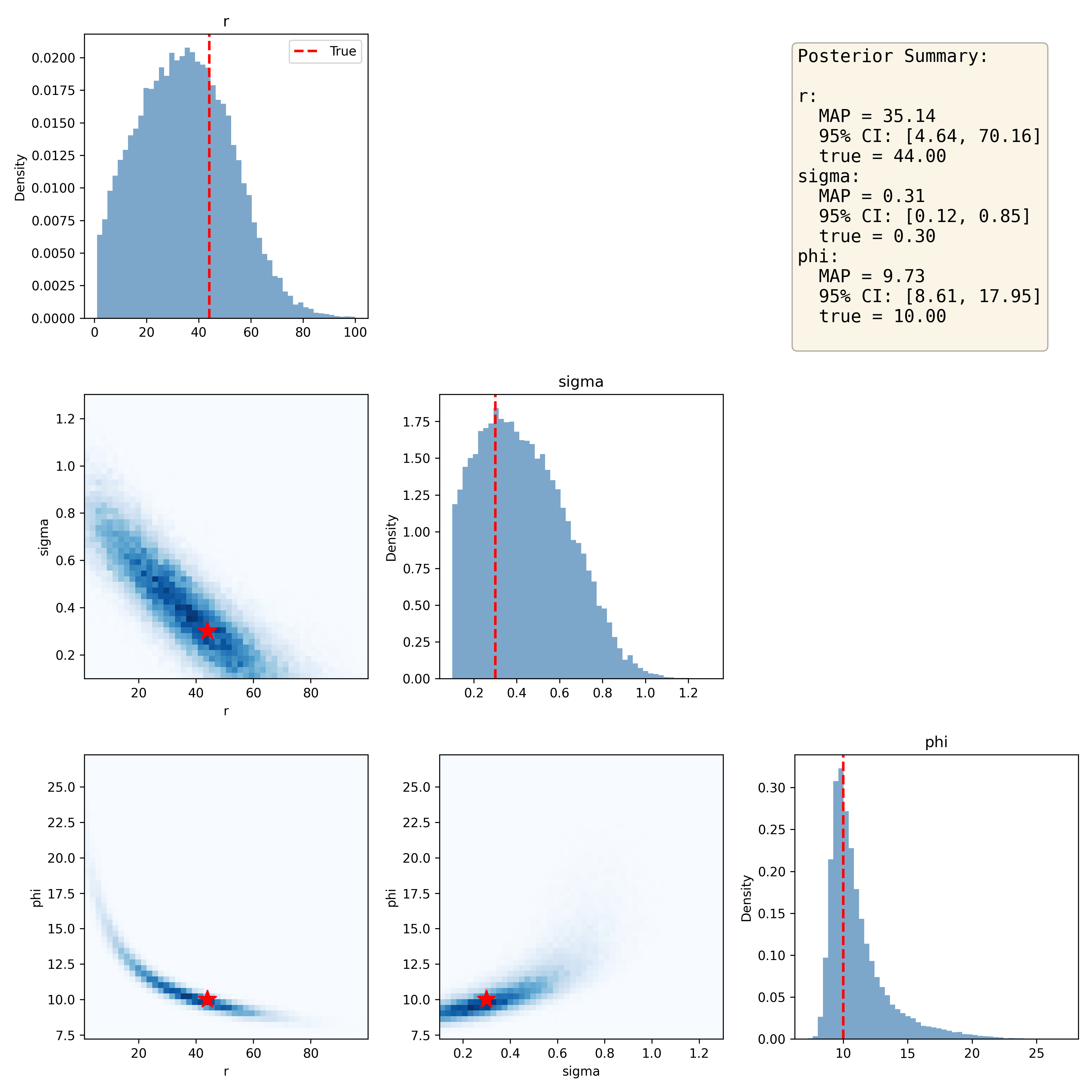
Figure 1. Joint distribution plots for the sampled posterior distributions of Ricker model parameters, with the true values denoted by the red star in the joint plots. The posterior summary presents the maximum a posteriori (MAP) estimate for each parameter along with the 95% credible interval based on the posterior distribution.
Parameter recovery
Simulation allows us to assess how well our estimation procedure performs, by generating data with known model parameters and then comparing the estimated parameters to the true values. Using the code that I had developed for the earlier example, I generated a simulation harness that ran a large number of simulations and recorded the results; the full code is here. I started by training the posterior estimator using one million simulations, in order to ensure that it had good training across the range of possible parameters; Given that this just needs to be trained once, I saved it for later use in my simulations. Then I performed 10,000 experiments in which I generated a dataset from the Ricker model based on known parameters along with added noise, and then used the posterior estimator to estimate the parameters for the dataset.
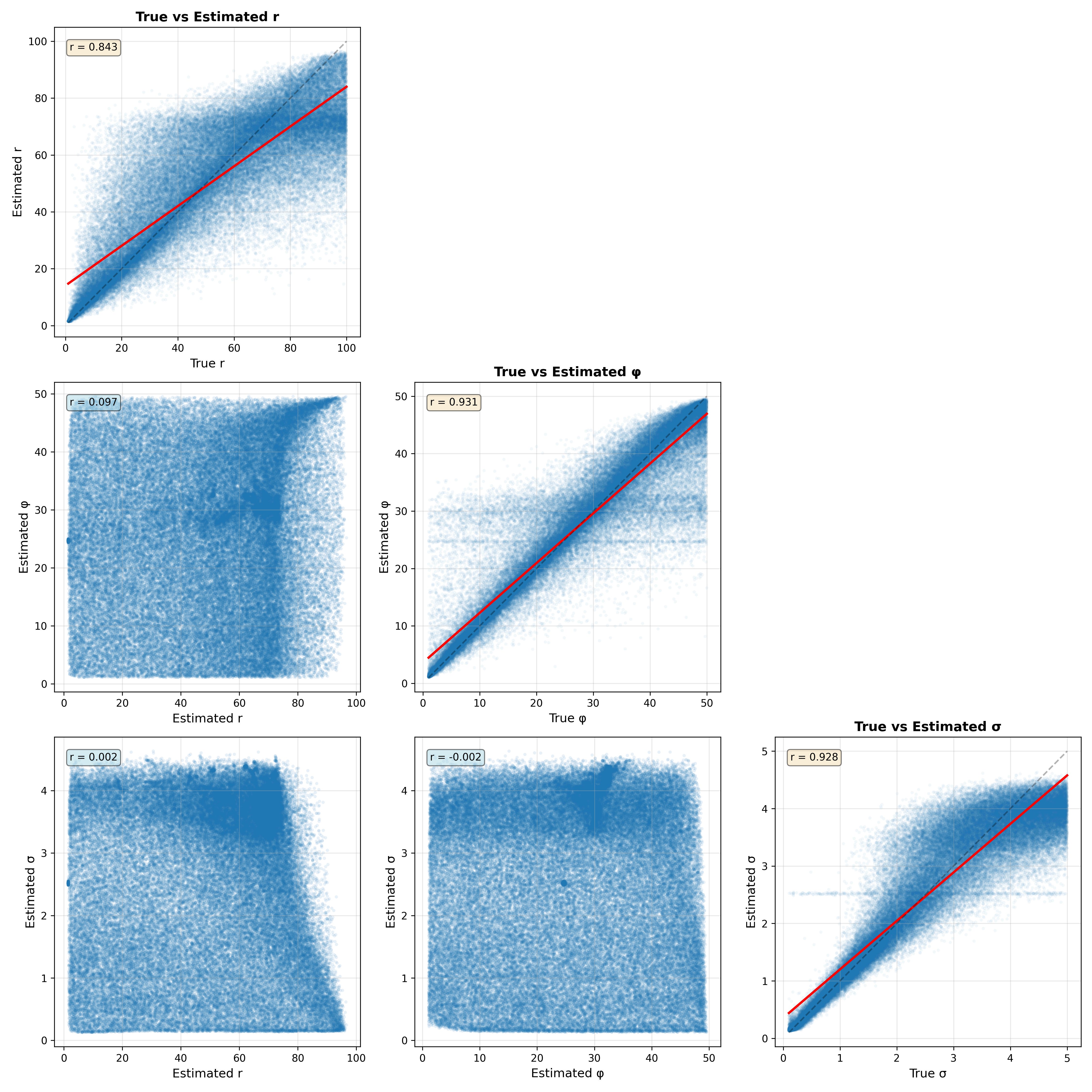
Figure 2. Parameter recovery analysis for 10,000 datasets generated from the Ricker model. The plots along the diagonal show the relationship between the true and estimated values and their correlation. The plots in the lower triangle show the relationship between parameter estimates for each pair of parameters.
Figure 2 shows the relationship between the true and estimated parameters on the diagonal. We see that the correlations between true and estimated parameters are reasonable but that in some rare cases the estimates can veer far from the true values. There is also faint evidence of some pathologies in model fitting. For both the phi and sigma parameters, there are bands of data points that suggest that the parameter estimation is being pulled towards the prior mean, which can occur if the data are not sufficiently informative. The off-diagonal plots show the relationship between the estimated parameters for each pair of parameters. This is useful to visualize because correlations between estimated parameters can reflect a lack of model identifiability, in which parameters trade off against one another. In this case these relationships are very weak, suggesting that the model parameters are indeed identifiable.
In the next post I will turn to a discussion of statistical calibration using randomization.