Validating scientific software using simulations
Better Code, Better Science: Chapter 9, Part 1

This is a possible section from the open-source living textbook Better Code, Better Science, which is being released in sections on Substack. The entire book can be accessed here and the Github repository is here. This material is released under CC-BY-NC-ND.
So far I have focused very heavily on reproducibility, that is, the ability to generate the same answer when code is run repeatedly. However, it’s easy to reliably generate the wrong answer! In measurement theory there is a fundamental distinction between reliability and validity: Reliability means performing the same method repeatedly results in highly similar results, whereas validity refers to whether the estimated result is close to the true result. In this chapter we turn to the validation of scientific software, by which I mean the degree to which it performs the intended task as expected and gets the answers right.
Creating simulations
Creating simulations is perhaps the most important tool that computers offer the scientist, as captured in a well-worn quote by Press et al. in their Numerical Recipes book:
offered the choice between mastery of a five-foot shelf of analytical statistics books and middling ability at performing statistical Monte Carlo simulations, we would surely choose to have the latter skill. (p.691)
Simulations are indeed a powerful way to understand a system even when it’s not analytically tractable. More importantly, they are generally the only way that we can establish ground truth against which we can compare our models. As scientists we never know the true process that generates our data, but with simulations we can have complete control over the data generation process.
My previous book, Statistical Thinking gives an overview of how to use simulations in the context of statistics; here I will focus primarily on the use of simulation in the context of software validation, but I recommend that book for background reading if you aren’t already familiar with the concept of a statistical distribution.
Generating random numbers
The most fundamental requirement in nearly any simulation is the ability to generate random numbers.1 What makes a series of numbers random is that it is impossible (or at least nearly impossible) to predict the next value in the series. Random numbers are defined by the distribution that characterizes them, which is a mathematical function that describes the “shape” of the data when they are summarized according to the relative frequency of different values or ranges of values. Picking the correct distribution is essential to ensure that any simulation performs as advertised. Fortunately, there are lots of existing packages that provide tools to generate random numbers for nearly any distribution; we will focus on the NumPy package here since it is the most commonly used.
The simplest distribution is the uniform distribution, in which any possible value (within a particular range for continuous values) has the same probability of occurring. We can generate uniform random variates by first creating a random number generator object using np.random.default_rng(), and then calling rng.uniform() which returns random samples from the distribution:
rng = np.random.default_rng()
rng.uniform(size=10)
array([0.56449692, 0.6880841 , 0.43249236, 0.28950554, 0.02708363,
       0.61239335, 0.30663968, 0.3854357 , 0.57454511, 0.07974661])
In this case, rng.uniform() by default generates floating point values that fall within [0, 1]; this can be changed using the location and scale parameters to the function. If we generate a large number of these then we can create a distribution plot (often called a histogram) showing how the numbers are distributed, as shown in Figure 1.
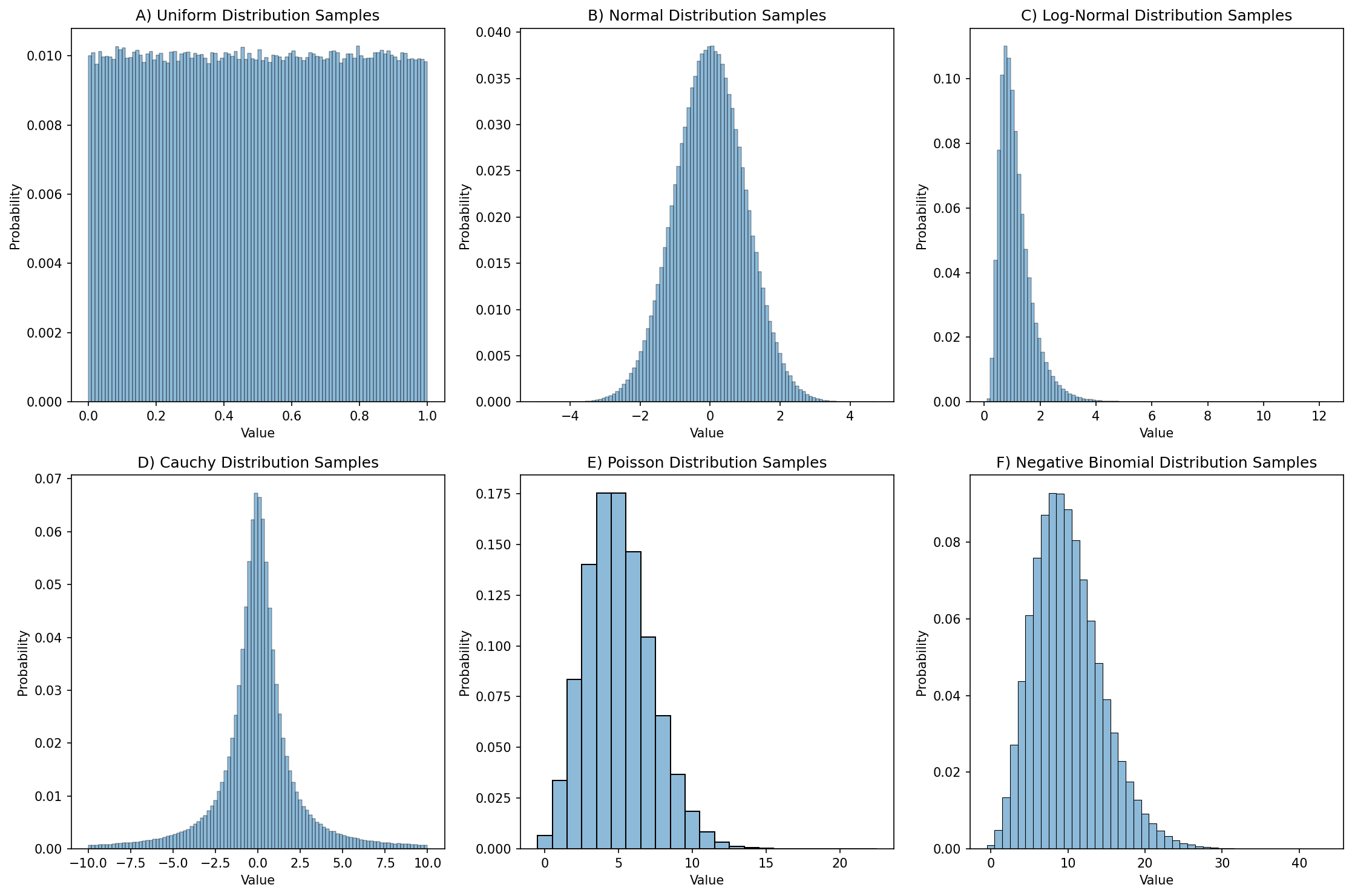
Figure 1. Distribution plots for 1,000,000 random samples from each of six different distributions.
For purposes of reproducibility it’s often useful to be able to regenerate exactly the same series of random samples. We can do this by specifying a random seed, which gives the random number generating a starting point. If you are going to do simulations then it is important to understand the specific random number generator that your code will use. This blog post provides an excellent introduction to the NumPy random generation system; here I will only give a brief overview. Previously it was common to use the global NumPy random seed function (np.random.seed()) to set the seed, and this is still necessary when using packages that access the global random number generator. However, the best practice is to generate a random number generator object (using np.random.default_rng()), and then call the methods of that object to obtain random numbers, as I did above. This prevents surprises in case other functions modify the global seed, helps isolate your specific generator, and enables multiple parallel generators. Here is an example:
rng = np.random.default_rng(seed=42)
rng.uniform(size=4)
array([0.77395605, 0.43887844, 0.85859792, 0.69736803])
If we run this again, we see that a different series of numbers is generated:
rng.uniform(size=4)
array([0.09417735, 0.97562235, 0.7611397 , 0.78606431])
However, if we generate another object with the same seed, we will see that it gives us the same values as above:
rng2 = np.random.default_rng(seed=42)
rng2.uniform(size=4)
array([0.77395605, 0.43887844, 0.85859792, 0.69736803])
rng2.uniform(size=4)
array([0.09417735, 0.97562235, 0.7611397 , 0.78606431])
Setting random seeds is important to enable exact reproducibility of results generated using random numbers. However, it’s also important to ensure that one’s results are robust to the choice of random seed, as I will discuss later in the context of machine learning analyses.
Choosing a distribution
Choosing the right distribution for a simulation often comes down to understanding the data-generating process and kind of data that are being modeled. Here are a few examples of distributions and their common use cases:
Discrete outcomes
Bernoulli: A distribution of binary outcomes (often interpreted as success vs failure) given a probability of a positive outcome.
Examples: Whether a patient responds to a given treatment, whether a hard drive fails within a particular period of time.
Binomial: A distribution of the number of successes across a specific number of Bernoulli trials, given a probability of a positive outcome.
Examples: The number of patients who respond to treatment in a clinical trial treatment group, the number of hard drives that fail within a particular period of time at a particular data center
Categorical: A distribution with several distinct possible outcomes, each of which has a particular probability:
Examples: Eye color across a population, programming languages used by programmers in a company
Uniform: A specific form of a discrete categorical variable with equal probability
Examples: equiprobable physical outcomes such as a dice roll.
Multinomial: A multivariate generalization of the binomial, representing the counts of multiple possible outcomes across a set of independent trials with fixed probabilities of each outcome.
Examples: Frequencies of types of stars in a galaxy, frequencies of cell types in a tissue sample
Continuous outcomes:
Uniform: A distribution with equal probability density for all values within the range.
Examples: probabilities of events when there is no prior knowledge, equiprobable continuous physical outcomes
Beta: A generalization of the uniform distribution that models the probability of values within a range but allows different values to have different probabilities.
Examples: Prior probabilities in a Bayesian model, proportions of time spent in a particular state.
Normal (or Gaussian): A symmetric distribution centered around a mean, which commonly arises when an outcome is generated based on many small additive contributions. The Central Limit Theorem explains why this occurs so frequently, as it should arise for sums of independent random variables sampled from any distribution, as long as the sample size is large enough and the distribution has finite variance.
Examples: Height of individuals in a population, measurement errors for continuous variables
Log-normal: Distribution of positive continuous values whose logarithm is normally distributed. It reflects the expected values of a product of independent random variables.
Examples: Wealth and income distributions in a population, biological growth processes
Count data:
Poisson: This is a distribution of counts of events within a fixed interval assuming that the events are independent and occur at a constant rate. Unlike the binomial there is no limit on the number of events that can occur, and it is the limiting case of the Binomial when the sample size nn approaches infinity and the probability pp approaches zero (and n∗pn∗p remains constant).
Examples: The number of atoms decaying within a particular period, the number of emails that a person receives within a day
Negative binomial: A distribution that models count data that are overdispersed, meaning that their variance is greater than their mean. It can also be interpreted as representing the number of failures that occur before a given number of successes.
Example: Commonly used in genomics to model read counts in genomic sequencing.
Waiting time data:
Exponential: A distribution of waiting times in a process governed by a Poisson distribution, with a constant hazard rate (i.e. the probability of happening in the next period is independent of whether the event has happened yet).
Examples: Time between atomic decays, time between hard drive failures
Weibull: A generalization of the exponential distribution that allows modeling of waiting times with increasing, constant, or decreasing hazard rates.
Examples: Response times in human behavior, time to failure for some electronic devices
It is essential to choose the right distributions for a simulation; otherwise the results may be misleading at best or meaningless at worst.
In the next post I will discuss how to simulate data from a mathematical model,
For the sake of convenience I will use the term random numbers for series of numbers generated by a computational algorithm, but it is more precise to call them pseudorandom numbers, because the series will ultimately repeat after a very long time. See Chapter 3 of Knuth’s Seminumerical Algorithms (Vol. 2 of The Art of Computer Programming) for a detailed discussion.